5. HMM Explanation and its Application to GWAS
a. HMM Walkthrough in terms of Weather
Imagine that it’s raining in some places and sunny in some other places. If we know that it’s raining in Saint Paul, it is more likely that it’s also raining rather than sunny in cities nearby Saint Paul. If we know that it’s sunny in LA, then we could to some extent safely assume that it’s more likely for cities close to it, e.g. San Francisco, to be sunny rather than rainy.
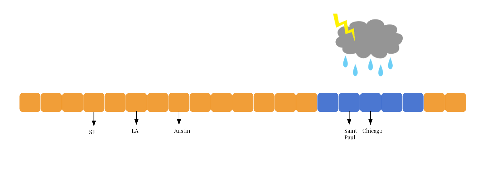
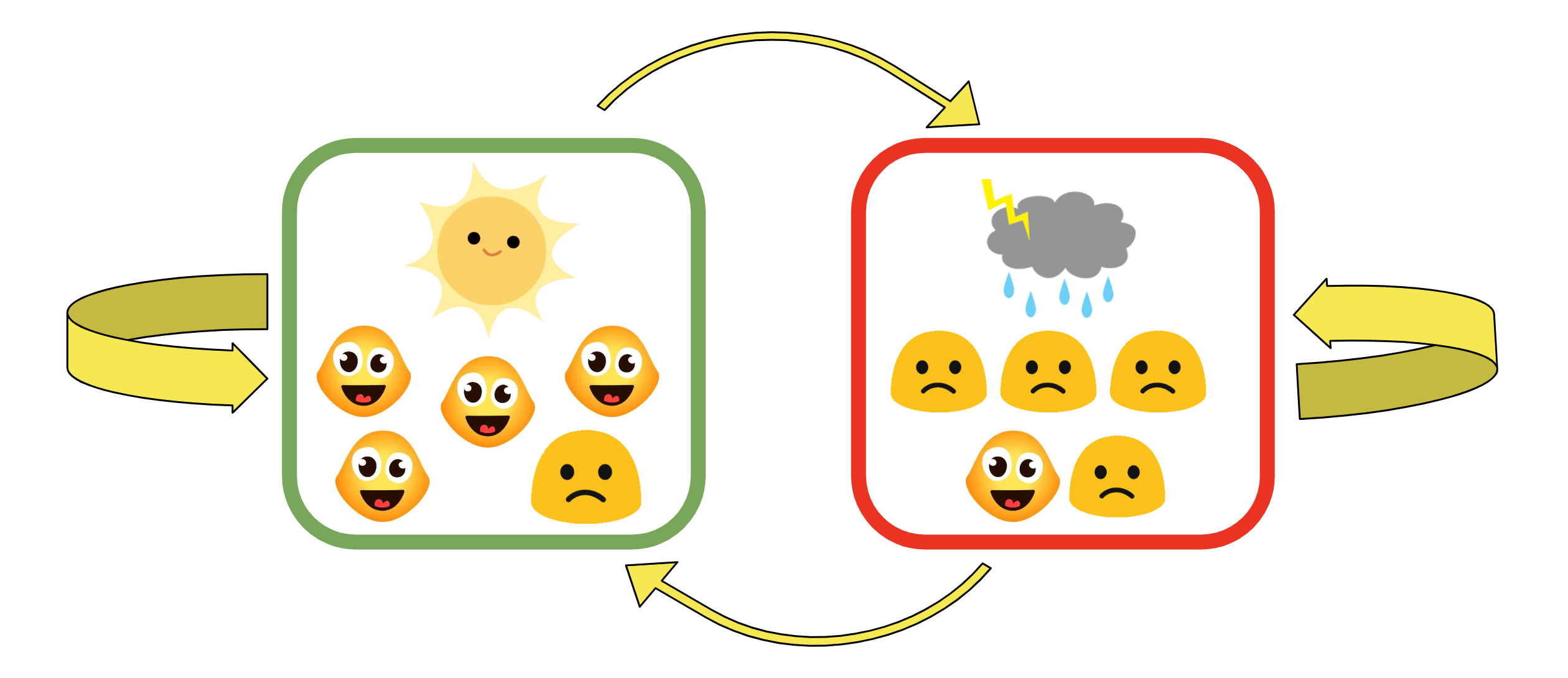
Therefore, using the Saint Paul - Chicago example, we know that if Saint Paul is sunny, then it’s more likely to be sunny in Chicago too, denoted by the thicker arrow. The chance that it’s rainy in Chicago given that it’s sunny in Saint Paul is gonna be low, denoted by the thinner arrow. These probabilities, represented by the thickness of arrows in the diagram below, are called transition probabilities, which simple mean the probability of maintaining in one weather state or transit to another one.
In this diagram, we also assume that sunny weather makes 80%(4/5) people happy and 20%(1/5) people sad, and rainy weather makes 80%(4/5) sad and 20%(1/5) happy. These probabilities are called the omission probabilities, which are the probabilities of observing a specific mood given the weather(the hidden state). For example, we can say the probability of observing a happy person in a city that is raining is assumed to be 20%.
Then here’s a question we need to consider:
What do we do if we don’t know the exact probabilities denoted by the yellow arrows above?
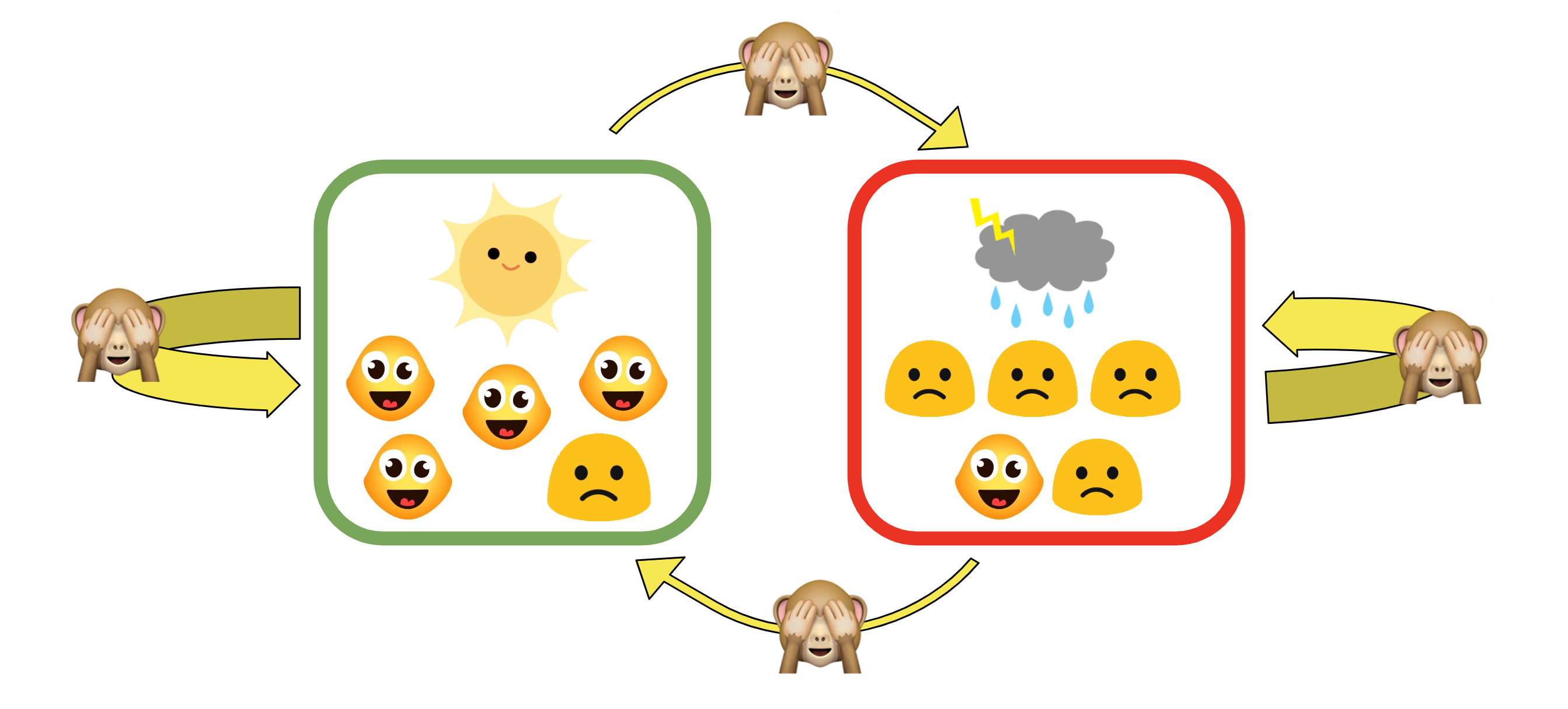
In real data, this is the case for most of the time. A method that we will show in the Demo section in the GWAS is called EM algorithm (Ephraim and Merhav 2002), which looks at all of our observed data and infers these probabilities.
Putting all of these together, we consider the question:
Given that we know the mood of one person living in each city and have assumed the chances of getting different moods given different weather states, can we determine whether it’s rainy or sunny in different cities?
The moods of the people are the observed state, and the weather we need to determine for each city is called the hidden state. This is essentially the idea behind Hidden Markov Model.
b. How does it play out in GWAS?
In the paper “Multiple testing in genome-wide association studies via hidden Markov models” by Zhi Wei, Wenguang Sun, Kai Wang, and Hakon Hakonarson (Wei et al. 2009), they designed a procedure to use hidden markov model to incorporate the correlations among SNPs into account in GWAS, and they named it the PLIS procedure.
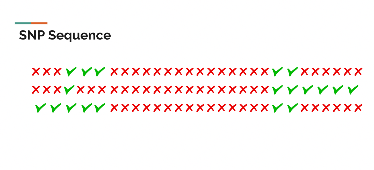
Imagine this is a section of a person’s genome, which each icon representing a single nucleotide polymorphism(SNP). For some certain trait, suppose the green check mark means this SNP is associated with the trait, and the red false mark indicates this SNP is not associated with the trait. Since SNPs are highly correlated as we learnt from the heatmap for Linkage Disequilibrium, if a SNP is associated with some trait, then its next SNP would be more likely to be also associated with the trait than not, and vice versa.
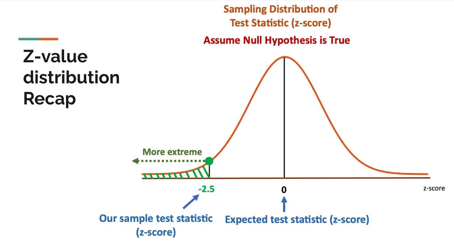
In statistics, z-values measure the distance between some random variable and the mean. Generally speaking, when we assume the null hypothesis is true, the expected value of z-values is zero and z-values follow a standard normal distribution by its definition. On the other hand, when the null hypothesis is rejected, the z-values would follow some other kinds of distribution.
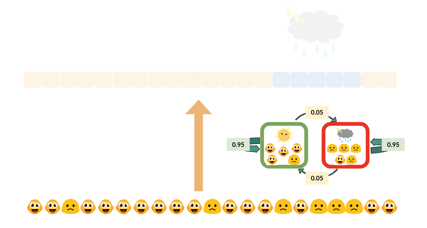
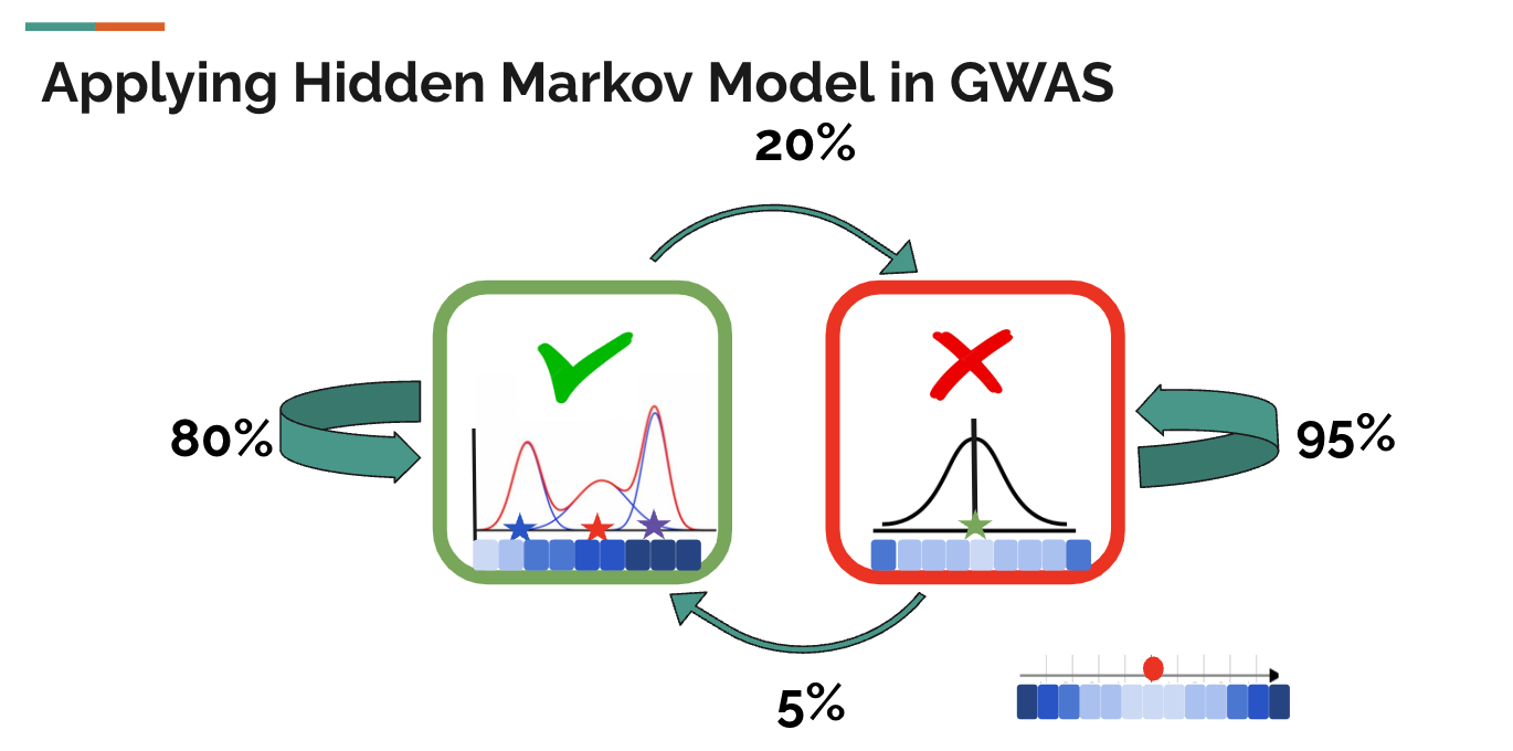
With the background knowledge of z-values, and the intuition of the correlation among nearby SNPs, we can come back to see a simple diagram of a hidden markov model in GWAS. Still, the green check mark means the SNP is associated with the trait, and the red false mark means the SNP is not associated with the SNP. In the example diagram below, if a SNP is associated with some trait, then the probability that its next SNP(by physical position) is also associated with the trait is 80%, and the probability that its next SNP is not associated with the trait is only 20%. If a SNP is not associated with the trait, then there is a 95% probability that the next SNP is also not associated with the trait and only a 5% probability that the next SNP is associated with the trait. This should match our intuition from the SNP sequence above and the how linkage disequilibrium works.
In Hidden Markov Models(HMM), these probabilities (80%, 20%, 95%, 5%) are called transition probabilities, which means the probability to maintain the same hidden state or transit to the other hidden state.
Apart from that, we also have observed states in hidden markov models, which are the z-values in the PLIS procedure. The PLIS procedure assumes that when the SNP is not associated with the trait, the z-values follow a standard normal distribution, and when the SNP is associated with the trait, the z-values follow some normal mixture, which is simply the summation of different normals.
When given the hidden states, the probability of getting an observed state is called the omission probability. Here, the omission probability of getting a z-value that is far from zero is higher when the SNP is associated with the trait than when the SNP is not. Stated differently, the omission probability of getting a z-value that is close to zero is higher when the SNP is not associated with the trait than when the SNP is associated with it.
Note: the blue blocks represent z-values. The darker the blue is, the farther away this z-value is from zero.
However, as we only have observed states (z-values) in this GWAS, we actually don’t know the transition probabilities. Fortunately, for any hidden markov model, the expectation-maximization(EM) algorithm can be used to infer the transition probabilities from the sequence of observed z-values. The PLIS procedure applied it to infer the transition probabilities as well.
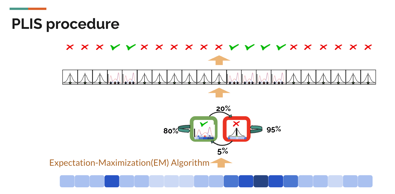
As the diagram shows above, the PLIS procedure starts only with one observed state for each SNP- the z-value. Given the z-value sequence for each chromosome, the Expectation-Maximization(EM) algorithm can give us the optimal set of transition probabilities of the hidden markov model for each chromosome that makes our observed sequence of z-values most likely to have occured. At the same time, it would give us the estimated/predicted distribution of z-values and a test statistic called LIS for each SNP.
LIS is defined as \(LIS_i\) = P(\(SNP_i\) is not associated with the trait | observed sequence of z-values ). In other words, it is the probability that a case is a null given the observed data. In a way, LIS is defined just like p-value was, and the smaller the LIS is, the more significance this SNP shows toward the trait.
The conventional p-value procedure is simple doing marginal regressions on each SNP and rank the importance of SNPs by ranking their p-values from small to large. To deal with the multiple testing problem, we can use Bonferroni’s Correction to choose a smaller cut-off threshold of those p-values to determine which SNPs are associated with the trait and which ones are not.
To some extent, the test statistic LIS works in the same way. We can also rank SNPs’ importance by ranking LIS from small to large. As for how to choose a cutoff threshold, we can conduct the LIS procedure as follows.
Denote the ordered LIS values by \(LIS_1\), \(LIS_2\), …, \(LIS_m\), and the corresponding hypotheses by \(H_1\), \(H_2\), …, \(H_m\). The LIS procedure operates as: Let \(l = max\{i:\frac{1}{i}\sum_{j=1}^{i}LIS_j\leq\alpha\}\), then reject all \(H_i\) for \(i = 1,...,l\).
With the LISs and the cut-off threshold derived from the LIS procedure described above, PLIS gives the hidden states of all SNPs, which is what we actually care about - controlling for the global false discovery rate at \(\alpha\), whether the SNPs are associated with the trait or not.
Note: The PLIS procedure should be applied to chromosomes one by one because it assumes the independency of different chromosomes.