3. Multiple Testing, and common correcting procedures
a. What does Multiple Testing look like in GWAS?
In order to find the association between the disease and SNP, we can do our familiar linear regression, where the disease is \(y\) and the SNPs are the predictors. However, this is not feasible in GWAS because the number of columns representing SNPs is greater than the number of rows of observations. For this reason, we cannot determine the model coefficients. If we run it, it’s gonna be all NAs. We can determine the coefficients of the SNPs at the very beginning, but then when the number of columns exceed the rows, it’s gonna be all NAs due to lack of information to infer the coefficients.
Because of that, we have to do marginal regression, which means that we have to fit the linear regression separately for each of the SNP in the dataset.
\[\text{Disease} \sim lm(SNP_i , \space data=data) \text{ for i ranges from 1 to n SNPs in the dataset}\] The fact that we have to run this regression \(n\) times is an example of Multiple Testing in GWAS. This leads to increasing chance of Type 1 error, which is to reject the null when the null is true. Here’s a little real life situation about Type 1 error.

That leads us to the question: How can we reduce Type 1 Errors in Multiple Testing?
b. Correcting Methods for Multiple Testing
There are two types of procedures used to correct for Type 1 Errors in Multiple Testing: Bonferroni Correction and Simulation-based Approach.
i. Bonferroni Correction
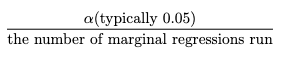
Bonferroni Correction is very popular approach in which we obtain our new p-value threshold by dividing our desired alpha (0.05) by the number of tests we’re conducting.
A drawback of the Bonferroni Correction is that it operates under the assumption that all SNPs are independent and provide a very conservative p-value cut-off, which can increase the chance of getting Type 2 Errors, which is the probability of not finding a correlation when there is one. As we go along in the introduction, you’ll know why this assumption is not a valid on in GWAS.
ii. Simulation-based Approach
In Simulation-based Approach, we simulate a null trait, which is a trait that’s not associated with any of the SNPs. After that, we use GWAS and record the smallest p-values, and we repeat this process around 500-1000 times. Our new p-value threshold is the cut-off value at the lowest 5th percentile.
A drawback of the Simulation-based Approach is that it is very computationally extensive, which requires a lot of resources when dealing with a large number of SNPs in GWAS.
In order to understand why the fix for Type 1 error is not that straightforward in GWAS, we’re going to look at the concept of Linkage Disequilibrium and understand more of the context behind the method that we’re researching in this project.
3. Linkage Disequilibrium
Linkage Disequilibrium (LD) is the correlation between nearby variants that cause the alleles at close polymorphisms (seen on the same chromosome) to be associated within a population more frequently than they would be if they weren’t linked (Holloway and Prescott 2017). In other words, SNPs are more correlated if they are closer in terms of distance.
This is a SNP matrix. The diagonal line indicates the position on the matrix where the SNP is itself. The more orange the color radiant is, the more correlated the SNPs are to one another. Since the orange is concentrated mostly in the area surrounding the diagonal line, it shows that SNPs that are closer to one another are more correlated. Therefore, if the causal SNP is missing, we are very likely to detect a high association between the nearby SNPs and the disease. With this knowledge of LD in mind, using Bonferroni Correction won’t yield accurate results. Since the p-value threshold determined by this method is very conservative, the chance of getting Type 2 errors will increase. Because there are a lot of SNPs, using Simulation-based Approach requires a great deal of resources due to the large number of SNPs involved.
Where does LD come from?
LD is the result of recombination, which is an exchange in genetic material to form a new pair of chromosomes for the offspring. Specifically, the offspring inherits the genetic materials from both parents, but not in the exact order as the parents’ chromosomes. Either or both of the chromosomes from each parent’s chromosome pair will “recombine” through cross-over, as observed in this diagram.
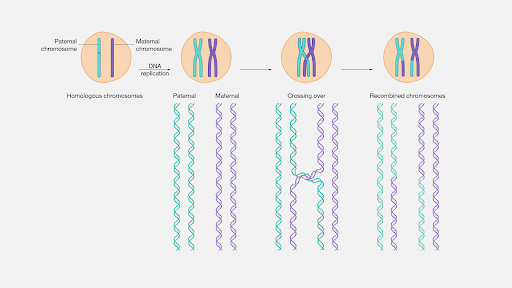
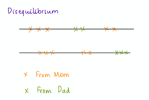
Since linkage is the probability that two segments of DNA are inherited together, SNPs that are closer in terms of distance on the chromosome are more likely to be inherited together. As the SNPs are not independently distributed and uniformly distanced on the chromosome, there’s a disequilibrium.
The method we research, Pooled Local Index of Significance (PLIS) accounts for the correlation between SNPs using Hidden Markov Model, which follows in the next section.