Please refer to the simulation at this link to see our step-by-step simulation for the PLIS method for one iteration (Wei et al. 2009): https://bookdown.org/jguan/Simulation/
Running the simulation for fifty iterations
As we have seen in the last six steps, we only randomly chose one set of four SNPs to be causal SNPs and compared the sensitivity of PLIS procedure and conventional p-value procedure(with logistics regression). However, the higher sensitivity of PLIS procedure based on only one case is not convincing at all, because it could just be a coincidence. Thus, we decided to run randomly choose 50 sets of four SNPs and perform simulation for all 50 situations, then we can calculate the average of both methods’ sensitivity and compare their performance based on a more convincing result.
Setting up
#Uncomment the following lines if you haven't installed snpStats
#if (!require("BiocManager", quietly = TRUE))
    #install.packages("BiocManager")
#BiocManager::install("snpStats")hapmap <- read.plink(bed, bim, fam)Here is a function to calculate z values based on p-values and odds_ratio.
calculate_zvalue = function(p_value,odds_ratio){
# Creat a new vector to store all Z-scores of the two-tailed z-test
ZSCORE = c()
# Find the z-score for each SNP
  for (i in 1:length(p_value)) {
    # If Odd Ratio > 1, z-score is the integrated area above the p-value
    if((!is.na(odds_ratio[i])) && (odds_ratio[i]>1)){
      ZSCORE[i] = qnorm(p_value[i]/2,0,1,lower.tail=FALSE)
    }
    # Otherwise, z-score is the integrated area below the p-value
    else{
      ZSCORE[i] = qnorm(p_value[i]/2,0,1,lower.tail=TRUE)
    }
  }
# Append z-score to our dataset
return(ZSCORE)
}# How many SNPs from each chromosome you want to include in your dataset
SNPS = 2000# Get all snps you want to include to include in your dataset
startrow = 1
rowidx = c()
newmap = c()
for (i in c(1:2)){
newmap = rbind(newmap, hapmap$map[(startrow:(startrow+(SNPS-1))),])
rowidx = cbind(rowidx, startrow:(startrow+SNPS-1))
startrow = startrow + nrow(hapmap$map %>% filter(chromosome==i))
}Run the whole process of calculating sensitivities for 50 times.
#pick four causal SNPs for the disease, make sure two of them are nearby from one chromosome and the other two are far away from another chromosome

#index of causal SNPs

for(i in c(1:50)){

  hapmap <- read.plink(bed, bim, fam, select.snps = rowidx)

  #get the index of SNPs whose MAF is zero to exclude monomorphic SNPs
  mono <- which(col.summary(hapmap$genotype)$MAF == 0)

  #nomonosnps contain snps that are not monomorphic
  nomonosnps = hapmap$genotypes[,-mono]

  #nomonosnps is a SnpMatrix, let's convert it to a matrix for later use
  X <- as(nomonosnps, "numeric")


  causal_idx = c(causal_chr1_list[i],causal_chr1_list[i]+1,causal_chr2_list[i],causal_chr2_list[i]+800)

  # set the intercept value and effect size, suppose all 4 causal SNPs have the same effect to causing this fake disease
beta0 = -3
effect_size = log(1.5)

#Get the probability of having the disease for all 165 people
nom = exp(beta0 + effect_size*rowSums(X[,causal_idx]))
prob = nom/(1+nom)

#Check the probabilities
#prob

#if the probability of having the disease is larger than 0.5, we assign this person's disease status to 1, and vice versa
status = c()
for (i in 1:length(prob)){
  status = cbind(status, as.numeric((!is.na(prob[i])) && prob[i] > 0.5))
}


p = c()
or = c()
for (col in (1:ncol(X))){
  #short for SNP minor allele count
  SNPmac = as.vector(X[,col])
  #convert status into a vector
  statusv = as.vector(status)
  #fit a logistic regression model
  model.glm <- glm(statusv ~ SNPmac, family = 'binomial')
  #beta0 is the intercept of the logistic regression
  beta0 = summary(model.glm)$coefficients[1,1]
  #beta1 is the coeff of increment of 1 minor allele's effect on the log(p/1-p) = log(odds_ratio)
  beta1 = summary(model.glm)$coefficients[2,1]

  or = cbind(or,exp(beta1))
  p = cbind(p, summary(model.glm)$coefficients[2,4])

}
or = as.vector(or)
p = as.vector(p)

#Apply the method above to calculate z-values based on p-values and odds ratios
z = calculate_zvalue(p,or)

# exclude monomorphic SNPs
useful_snps = hapmap$map[-mono,]

# build a dataframe with snp.name, chromosome, position, p-values, odds_ratios, and z-values, then remove the causal SNPs by their row index
df = data.frame(snp.name = useful_snps$snp.name, chromosome = useful_snps$chromosome, position = useful_snps$position, pvalue = p, odds_ratio = or, z_value = z) %>% filter(!row_number() %in% causal_idx)


# a simple function that checks if a number in list k is within the +/- n range to any number in a given list, return T/F only
nearby = function(k, list, n){
  near_list = c()
  for(i in k){ near = F
    for (j in list){ if( abs ( i - j ) <= n ){ near = T } }
    near_list = c(near_list, near)}
  return(near_list)
}

nearby_status = c()


nearby_status = c(nearby_status, nearby(seq(1,1780,1),causal_idx[1:2], n=10))
nearby_status = c(nearby_status, nearby(seq(1781,3578,1),causal_idx[3:4], n=10))

df$nearby_status = nearby_status


library(PLIS)
SNP = c()
LIS = c()
for (i in 1:2){
  #get the snps on chromosome i
  chr_sample=df[which(df[,"chromosome"]==i),]

  #make sure these snps are correctly ordered by their physical locations
  chr_sample <- chr_sample[order(chr_sample[,"position"]),]

  #calculate z values
  chr_sample$z = calculate_zvalue(chr_sample$pvalue, chr_sample$odds_ratio)

  #apply EM algorithm
  chr_sample.L2rlts=em.hmm(chr_sample$z, L = 2)

  #append new results
  SNP = rbind(SNP, chr_sample)
  LIS = c(LIS, chr_sample.L2rlts$LIS)
}

# plis controls the global FDR at 0.01 here for the pooled hypotheses from different groups
plis.rlts=plis(LIS,fdr=0.001)

# gFDR stands for global FDR, denotes the corresponding global FDR if using the LIS statistic as the significance cutoff
all.Rlts=cbind(SNP, LIS, gFDR=plis.rlts$aLIS, fdr001state=plis.rlts$States)


count_near_chra = sum((df%>%filter(chromosome==1))$nearby_status)
count_near_chrb = sum((df%>%filter(chromosome==2))$nearby_status)
count_near = sum(df$nearby_status)

sensitivity_lis = c()
for (i in 1:10){
  LIS_rank = all.Rlts[order(all.Rlts[,"LIS"])[1:(i*100)],]
  sensitivity_lis = c(sensitivity_lis, sum(LIS_rank$nearby_status)/count_near)
}
lis = cbind(lis, sensitivity_lis)


sensitivity_lis_a = c()
for (i in 1:10){
  LIS_rank = all.Rlts[order(all.Rlts[,"LIS"])[1:(i*100)],]
  sensitivity_lis_a = c(sensitivity_lis_a, sum((LIS_rank%>%filter(chromosome==1))$nearby_status)/count_near_chra)
}
lisa = cbind(lisa, sensitivity_lis_a)

sensitivity_lis_b = c()
for (i in 1:10){
  LIS_rank = all.Rlts[order(all.Rlts[,"LIS"])[1:(i*100)],]
  sensitivity_lis_b = c(sensitivity_lis_b, sum((LIS_rank%>%filter(chromosome==2))$nearby_status)/count_near_chrb)
}
lisb = cbind(lisb, sensitivity_lis_b)

sensitivity_p = c()
for (i in 1:10){
  p_rank = all.Rlts[order(all.Rlts[,"pvalue"])[1:(i*100)],]
  sensitivity_p = c(sensitivity_p, sum(p_rank$nearby_status)/count_near)
}
pmethod = cbind(pmethod, sensitivity_p)

sensitivity_p_a = c()
for (i in 1:10){
  p_rank = all.Rlts[order(all.Rlts[,"pvalue"])[1:(i*100)],]
  sensitivity_p_a = c(sensitivity_p_a, sum((p_rank%>%filter(chromosome==1))$nearby_status)/count_near_chra)
}
pa = cbind(pa, sensitivity_p_a)

sensitivity_p_b = c()
for (i in 1:10){
  p_rank = all.Rlts[order(all.Rlts[,"pvalue"])[1:(i*100)],]
  sensitivity_p_b = c(sensitivity_p_b, sum((p_rank%>%filter(chromosome==2))$nearby_status)/count_near_chrb)
}
pb = cbind(pb, sensitivity_p_b)

}
Calculate the average of sensitivities across both procedures and different chromosomes.
lis = rowMeans(lis)
lisa= rowMeans(lisa)
lisb = rowMeans(lisb)
pmethod = rowMeans(pmethod)
pa = rowMeans(pa)
pb = rowMeans(pb)
k = seq(100, 1000, 100)
lis_df = data.frame(top_k = k, value = as.vector(lis), type = 'PLIS Method', causal = 'both')
lis_a_df = data.frame(top_k = k, value = as.vector(lisa), type = 'PLIS Method', causal = 'nearby causal')
lis_b_df = data.frame(top_k = k, value = as.vector(lisb), type = 'PLIS Method', causal = 'far-away causal')
pval_df = data.frame(top_k = k, value = as.vector(pmethod), type = 'p-value Method', causal = 'both')
pval_a_df = data.frame(top_k = k, value = as.vector(pa), type = 'p-value Method', causal = 'nearby causal')
pval_b_df = data.frame(top_k = k, value = as.vector(pb), type = 'p-value Method', causal = 'far-away causal')
lis_p_comparison = rbind(lis_df,lis_a_df,lis_b_df, pval_df,pval_a_df,pval_b_df)
lis_p_comparison
top_k value type causal
1 100 0.1550000 PLIS Method both
2 200 0.2418750 PLIS Method both
3 300 0.3090625 PLIS Method both
4 400 0.3643750 PLIS Method both
5 500 0.4056250 PLIS Method both
6 600 0.4409375 PLIS Method both
7 700 0.4771875 PLIS Method both
8 800 0.5059375 PLIS Method both
9 900 0.5303125 PLIS Method both
10 1000 0.5506250 PLIS Method both
11 100 0.1390909 PLIS Method nearby causal
12 200 0.2318182 PLIS Method nearby causal
13 300 0.2836364 PLIS Method nearby causal
14 400 0.3318182 PLIS Method nearby causal
15 500 0.3690909 PLIS Method nearby causal
16 600 0.4027273 PLIS Method nearby causal
17 700 0.4363636 PLIS Method nearby causal
18 800 0.4627273 PLIS Method nearby causal
19 900 0.4763636 PLIS Method nearby causal
20 1000 0.4954545 PLIS Method nearby causal
21 100 0.1633333 PLIS Method far-away causal
22 200 0.2471429 PLIS Method far-away causal
23 300 0.3223810 PLIS Method far-away causal
24 400 0.3814286 PLIS Method far-away causal
25 500 0.4247619 PLIS Method far-away causal
26 600 0.4609524 PLIS Method far-away causal
27 700 0.4985714 PLIS Method far-away causal
28 800 0.5285714 PLIS Method far-away causal
29 900 0.5585714 PLIS Method far-away causal
30 1000 0.5795238 PLIS Method far-away causal
31 100 0.1556250 p-value Method both
32 200 0.2093750 p-value Method both
33 300 0.2446875 p-value Method both
34 400 0.2662500 p-value Method both
35 500 0.2946875 p-value Method both
36 600 0.3181250 p-value Method both
37 700 0.3387500 p-value Method both
38 800 0.3559375 p-value Method both
39 900 0.3746875 p-value Method both
40 1000 0.3940625 p-value Method both
41 100 0.1454545 p-value Method nearby causal
42 200 0.1918182 p-value Method nearby causal
43 300 0.2300000 p-value Method nearby causal
44 400 0.2490909 p-value Method nearby causal
45 500 0.2681818 p-value Method nearby causal
46 600 0.2827273 p-value Method nearby causal
47 700 0.3090909 p-value Method nearby causal
48 800 0.3245455 p-value Method nearby causal
49 900 0.3409091 p-value Method nearby causal
50 1000 0.3654545 p-value Method nearby causal
51 100 0.1609524 p-value Method far-away causal
52 200 0.2185714 p-value Method far-away causal
53 300 0.2523810 p-value Method far-away causal
54 400 0.2752381 p-value Method far-away causal
55 500 0.3085714 p-value Method far-away causal
56 600 0.3366667 p-value Method far-away causal
57 700 0.3542857 p-value Method far-away causal
58 800 0.3723810 p-value Method far-away causal
59 900 0.3923810 p-value Method far-away causal
60 1000 0.4090476 p-value Method far-away causalPlot the results
Stationary sensitivity trends without grouping by chromosomes
# Plot it using ggplot
ggplot(aes(x = top_k, y = value, color = type), data=rbind(lis_df,pval_df)) +
  geom_point(aes(group = seq_along(top_k)), size = 2) +
  geom_line() +
  scale_x_continuous(breaks = lis_p_comparison$top_k) +
  labs(x = 'SNP Ranking (Top K)', y = 'Value', color = 'Method Type') +
  theme_classic()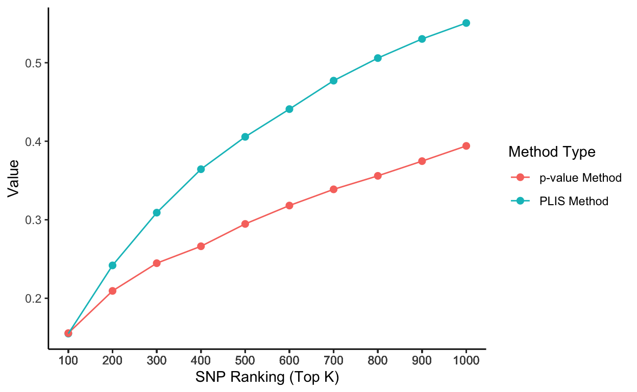
Stationary sensitivity trends grouped by chromosomes
# Plot it using ggplot
lisp_nfd = ggplot(aes(x = top_k, y = value, col = type, lty = causal), data=lis_p_comparison) +
  geom_point(aes(group = seq_along(top_k)), size = 2) +
  geom_line() +
  scale_x_continuous(breaks = lis_p_comparison$top_k) +
  labs(x = 'SNP Ranking (Top K)', y = 'Value', color = 'Method Type', lty = "chromosome") +
  theme_classic()

lisp_nfd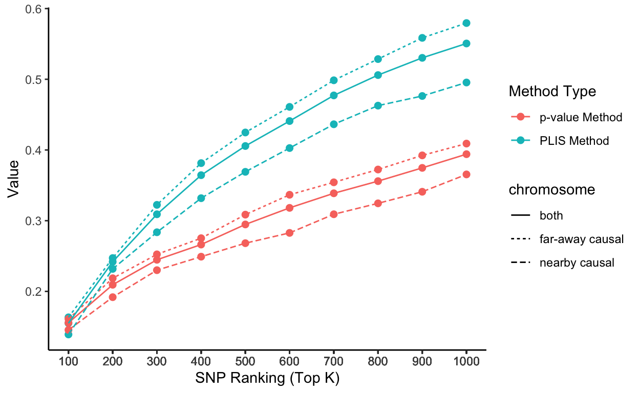
Animation
# Uncomment the following lines if you haven't installed the packages yet
# install.packages('gganimate')
# install.packages('transformr')
library(gganimate)
library(transformr)
lisp_nfd = ggplot(aes(x = top_k, y = value, col = type, lty = causal), data=lis_p_comparison) +
geom_point(aes(group = seq_along(top_k)), size = 2) +
geom_line() +
scale_x_continuous(breaks = lis_p_comparison$top_k) +
transition_reveal(top_k) +
ease_aes("linear") +
labs(x = 'SNP Ranking (Top K)', y = 'Value', color = 'Method Type') +
theme_classic()
animate(lisp_nfd, fps = 3, duration = 5)
anim_save("lisp_nfd.gif")